Communications Part 2:
STK Pro, STK Premium (Air), STK Premium (Space), or STK Enterprise
You can obtain the necessary licenses for this training by contacting AGI Support at support@agi.com or 1-800-924-7244.
This lesson requires STK 12.5 or newer to complete it in its entirety.
Capabilities covered
This lesson covers the following STK Capabilities:
- STK Pro
- Communications
Problem
You require a fast, easy way to set up and analyze communication systems prior to employing them in the field. You want to understand how to simulate radio frequency environmental phenomena such as rain and atmospheric absorption. You need to specify and measure the system's inherent noise characteristics. You want a way to take surrounding terrain into account such as hills and mountains which may be blocking your line of sight. Lastly, part of your system uses a servo system to steer an antenna and needs to be added to the analysis.
Solution
You will use STK to apply radio frequency (RF) atmospheric phenomena such as rain and atmospheric absorption to your link budget analysis. You will configure your receiver to account for and compute system noise temperature. Use local analytical terrain files to account for line of sight obstruction. Use a Sensor object to create a simple servo motor.
If you are new to STK, review the following Level 1 - Beginner tutorials first: Part 1: Build Scenarios and Part 2: Objects and Properties.
What you will learn
Upon completion of this tutorial, you will understand:
- How to add the ITU-R rain model and the ITU-R atmospheric absorption loss model in your scenario.
- How to create a medium transmitter on a LEO satellite.
- How to create a steerable ground site receiver antenna and a complex receiver model.
- How to simulate real-world RF situations with the system temperature interface and the terrain mask constraint.
- How to generate a simple and detailed link budget report.
Video guidance
Watch the following video. Then follow the steps below, which incorporate the systems and missions you work on (sample inputs provided).
Using the starter scenario (*.vdf file)
To speed things up and enable you to focus on this lesson's main goal, you will use a partially created scenario. The partially created scenario is saved as a visual data file (VDF) in your STK install.
Retrieving the starter scenario
- Launch STK (
 ).
). - Click (
 ) in the Welcome to STK dialog box.
 - Go to <STK install folder>\Data\Resources\stktraining\VDFs\.
- Select STK_Communications.vdf.
- Click .
Visual data files versus Scenario files
You must make sure that you save your work in STK as a scenario file (.sc) and not a visual data file (.vdf) by selecting Save As from the STK File menu. A VDF is a compressed version of an STK scenario, which makes them great for sending your work in STK to others. However, you want to use a scenario file while working with STK on your machine.
If you open a VDF file, STK keeps it as a VDF and does not automatically convert it to a scenario file. This means, STK does not change the file type of your scenario when you launch your scenario. You need to convert the VDF to a Scenario file using Save As.
Saving a VDF file as a Scenario file
Use Save As from the STK File menu to convert the VDF file that you opened into a scenario file.
- Open the File menu.
- Select Save As.
- Select the STK User folder on the left side of the Save As window.
- Click .
- Rename New Folder to match the title of the scenario.
- Open the folder you just created.
- Enter the name of the folder into File name field.
- Open the Save as type drop-down menu.
- Select Scenario Files (*.sc).
- Click .
Selecting relevant objects
In this scenario, you will analyze communications between a low earth orbit (LEO) satellite transmitter and a communications ground site receiver. The communications ground site is located in mountainous terrain. It employs a servo system that steers the antenna and is able to track the satellite. The satellite is in a repeating sun synchronous orbit.
You will only use a portion of the objects in the Object Browser, not all of them. There are extra objects because you can use this same scenario to complete other lessons about STK Communications.
- Select the check box for the following objects in the Object Browser:
- Communication_Site (
 )
) - LEO_Sat (
 )
) - Click Save (
 ). Save often during this lesson!
Configuring terrain and atmospheric models to your scenario
You will configure your scenario to include custom analytical terrain, the ITU-R rain model, and the ITU-R atmospheric absorption loss model. Later in this lesson, you will determine how these conditions affect your communications.
Loading custom analytical terrain
The Custom Analysis Terrain Sources table can be used to specify locally available terrain data files to be used for analysis and visualization.
- Right-click on your Scenario object (
 ) in the Object Browser.
 - Select Properties (
 ).
). - Select the Basic - Terrain page when the Properties Browser opens.
- Select the Use check box for PtMugu_ChinaLake.pdtt in the Custom Analysis Terrain Sources: list.
- Click to accept your change and to keep the Properties Browser open.
Loading the ITU-R Rain model
Environmental factors can affect the performance of a communications link. Apply rain and atmospheric absorption models to the analysis. Rain models are used to estimate the amount of degradation (or fading) of the signal when passing through rain. You will use an ITU-R rain model in your analysis.
- Select the RF - Environment page.
- Select the Rain, Cloud & Fog tab.
- Select the Use check box in the Rain Model frame. Leave the default ITU-R (International Telecommunication Union) model.
- Click to accept your change and to keep the Properties Browser open.
Loading the ITU-R Atmospheric Absorption model
Atmospheric Absorption models estimate the attenuation of atmospheric gases on terrestrial and slant path communication signals. In this case, you will use the default model: ITU-R Atmospheric Absorption model.
- Select the Atmospheric Absorption tab.
- Select the Use check box. Leave the default ITU-R model.
- Click to accept your changes and to close the Properties Browser.
Visualizing terrain in the 3D Graphics window
Display the PtMugu_ChinaLake.pdtt in the 3D Graphics window.
- Select the PtMugu_ChinaLake.pdtt check box in Globe Manager.
- Bring the 3D Graphics window to the front.
- Right-click on Communication_Site () in the Object Browser.
- Select Zoom To.
- Use your mouse to view the terrain affecting the communication site.

Communication Site and Terrain
Creating a medium transmitter
You will use the medium transmitter model on the LEO satellite. Unlike the simple transmitter model, the medium transmitter model provides more flexibility by letting you specify gain and power separately instead of entering their product (EIRP) directly. The medium transmitter model uses an isotropic, omnidirectional antenna, which is an ideal spherical pattern antenna with constant gain.
Inserting a Transmitter object
Attach a Transmitter (![]() ) object to LEO_Sat (
) object to LEO_Sat (![]() ).
).
- Select Transmitter (
 ) in the Insert STK Objects tool.
 - Select the Insert Default (
 ) method.
 - Click
- Select LEO_Sat () in the Select Object dialog box.
- Click .
- Right-click on Transmitter1 () in the Object Browser.
- Select Rename in the shortcut menu.
- Rename Transmitter1 () to Downlink_Tx.
Configuring the medium transmitter model
You will determine the properties of the Transmitter object.
- Open Downlink_Tx's () properties ().
- Select the Basic – Definition page when the Properties Browser opens.
- Click the Transmitter Model Component Selector (
 ).
). - Select Medium Transmitter Model in the Transmitter Models list once the Select Component dialog box opens.
- Click to accept your selection and to close the Select Component dialog box.
- Select the Model Specs tab.
- Set the following:
- Click to accept your changes and to close the Properties Browser.
| Option | Value |
|---|---|
| Power: | 10 dBW |
| Gain: | 20 dB |
| Data Rate: | 10 Mb/sec |
Adding a servo motor to the ground site receiver antenna
Your ground site receiver antenna is steerable. To create a steering device (e.g. servo motor) in STK, you use a Sensor (![]() ) object. A servo system is an automatic control system that, in this case, steers the ground antenna and points it at your target (e.g. LEO_Sat (
) object. A servo system is an automatic control system that, in this case, steers the ground antenna and points it at your target (e.g. LEO_Sat (![]() )).
)).
- Insert a Sensor (
 ) object using the Insert Default () method.
 - Select Communication_Site () in the Select Object dialog box.
- Click .
- Rename Sensor1 () to Servo_Motor.
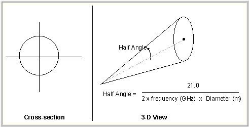
Half Power Sensor Patterns
Half Power sensor patterns are designed to visually model parabolic antennas. The sensor half angle is determined by frequency and antenna diameter.
HALF POWER SENSOR
- Open Servo_Motor's () properties ().
- Select the Basic - Definition page.
- Set the following:
- Click to accept your changes and to keep the Properties Browser open.
| Option | Value |
|---|---|
| Sensor Type: | Half Power |
| Diameter: | 3.5 m |
Raising the servo system's height
The servo system is 10 feet above the terrain. The location of the sensor is defined using a fixed displacement vector with respect to the parent object’s body frame. Later, when you attach the receiver to the sensor, the receiver's antenna will also be 10 feet above the terrain.
- Select the Basic - Location page.
- Open the Location Type: shortcut menu.
- Select Fixed.
- Enter -10ft in the Z: field. The parent object's (Communication_Site ()) positive Z point to the Earth's center. Therefore, to raise Servo_motor () above the ground, you use a negative value.
- Click .
Setting the pointing type to Targeted
The Targeted pointing type causes the sensor to point to other objects in the scenario.
- Select the Basic - Pointing page.
- Open the Pointing Type: shortcut menu.
- Select Targeted.
- Open the Track Mode: shortcut menu.
- Select Receive. The antenna is oriented slightly “behind” the current location of the LEO satellite. STK computes the appropriate amount by which to trail based on the light time delay.
- Move (
 ) LEO_Sat () from the Available Targets list to the Assigned Targets list.
 - Click to accept your changes and to close the Properties Browser.
Adding a complex receiver to the servo motor
You will use a Complex Receiver model on the ground communications site. The Complex Receiver model enables you to select among a variety of analytical and realistic antenna models and to define the characteristics of the selected antenna type.
Inserting a Receiver object
Insert a Receiver (![]() ) object and attach it to Servo_Motor (
) object and attach it to Servo_Motor (![]() ).
).
- Insert a Receiver (
 ) object using the Insert Default () method.
 - Select Servo_Motor () in the Select Object dialog box.
- Click to close the Select Object dialog box.
- Rename Receiver1 () to Downlink_Rx.
Configuring the Complex Receiver Model
- Open Downlink_Rx's () properties ().
- Select the Basic – Definition page when the Properties Browser opens.
- Click the Receiver Model Component Selector ().
- Select Complex Receiver Model in the Receiver Models list, when the Select Component dialog box opens.
- Click to accept your selection and to close the Select Component dialog box.
- Click .
LNA refers to Low Noise Amplifier. If you have those specifications, you can add them.
Configuring the receiver parabolic antenna
A parabolic antenna uses a parabolic mirror to focus incoming signals onto one reception point or direct the emissions of signals from a focal point into a directed beam.
- Select the Antenna tab.
- Select the Model Specs sub-tab.
- Click the Antenna Model Component Selector ().
- Select Parabolic in the Antenna Models list once the Select Component dialog box opens.
- Click to close the Select Component dialog box.
- Enter 3.5 m in the Diameter field.
- Click
Setting the RF environment to affect communications
Now that you have set up your STK objects and the surrounding environment, you will simulate how the environment will affect your communications. You will use the Receiver's System Noise Temperature and enable the Terrain Mask constraint.
Configuring the System Noise Temperature
The Receiver's System Noise Temperature allows you to specify the system's inherent noise characteristics. These can help simulate real-world RF situations more accurately.
- Select the System Noise Temperature tab.
- Select the Compute option. If you have specifications for your receiver, you can add them. For this analysis, use all the default settings.
- Select the Compute option in the Antenna Noise frame.
- Select the following:
- Sun
- Atmosphere
- Rain
- Cosmic Background
- Click .
Enabling the Terrain Mask constraint
The Terrain Mask constraint determines instantaneous visibility based on detecting intersections of the instantaneous line of sight with the terrain surface.
- Select the Constraints - Basic page.
- Select the Terrain Mask check box.
- Click to accept the changes and close the Properties Browser.
Generating a simple link budget
You will assess your communications with a simple link budget.
- Right-click on Downlink_Rx () in the Object Browser.
- Select Access… (
 ) in the shortcut menu.
 - Expand (
 ) LEO_Sat () in the Associated Objects list once the Access Tool opens.
 - Select Downlink_Tx ().
- Click
 .
. - Click in the Reports frame.
- Scroll to the right in the Link Budget report.
- Locate the C/N (dB), Eb/No (dB), and BER columns.
- Scroll down through the report.
- Close the Link Budget report.
Distance, rain and atmospheric absorption between the transmitter and receiver are causing fluctuations in your data.
Generating a detailed link budget
The Detailed Link Budget Report is a modified Link Budge Report with added Access Data Provider Elements.
- Click in the Access Tool.
- Select the Link Budget - Detailed (
 ) report in the Installed Styles list once the Report & Graph Manager opens.
 - Click .
- Scroll to the Atmos Loss (dB) and Rain Loss (dB) columns.
- Scroll down.
- Scroll to the right of the report and locate the C/N (dB), Eb/No (dB) and BER columns.
- Locate the Tatmos (K), Train (K), Tsun (K), Tcosmic (K), Tantenna (K) Tequivalent (K) columns.
You can see that the losses increase and decrease. Most losses occur when the satellite is low on the horizon. The signal has to pass through more atmosphere and is affected by rain and atmospheric absorption.
Rain and atmospheric absorption create loses in C/N and Eb/No and increase your BER.
They show data based on system noise temperature.
You can use this report to determine when you are receiving good communications from the satellite based on your system requirements.
Summary
This was an introduction to using medium transmitter and complex receiver models. You learned how to create a simple servo system used to track a LEO satellite with your receiver antenna. You learned how to apply rain models, atmospheric absorption models and analytical terrain to your analysis. You used a detailed link budget report that pulls data from more data providers than a simple link budget. Based on your analysis, you have determined that a viable communication link can be established between the satellite and the ground site.
Save your work
- Close any open reports, tools and properties.
- Save () your work.
What's next?
You are now ready to move onto the next tutorial Communications Part 3: Introduction to Analyzing Digital and Analog Transponders.